Thursday, July 30, 2026

Data Analysis of the World Happiness Report: Insights

Data Analysis of the World Happiness Report: Insights & Findings

What makes a nation happy? In this post, we analyze the World Happiness Report dataset using Python, pandas, and Seaborn. We'll explore dataset structures, handle missing values, inspect factor correlations, compare the happiest vs. least happy countries, and perform a deep-dive benchmark into Kenya's happiness metrics.


1. Data Loading & Preprocessing

The dataset contains 156 entries covering key socio-economic factors such as GDP per capita, social support, healthy life expectancy, freedom, generosity, and corruption perceptions.

import pandas as pd
import numpy as np

# Load the dataset
df = pd.read_csv('2018.csv')

# Impute missing 'Perceptions of corruption' value with median
if df['Perceptions of corruption'].isnull().any():
    median_corruption = df['Perceptions of corruption'].median()
    df['Perceptions of corruption'].fillna(median_corruption, inplace=True)
    print(f"Missing value imputed with median: {median_corruption:.3f}")

Statistical Summary of the Dataset

Metric Happiness Score GDP per Capita Social Support Healthy Life Exp. Freedom
Mean 5.376 0.891 1.213 0.597 0.455
Std Dev 1.120 0.392 0.302 0.248 0.162
Min 2.905 0.000 0.000 0.000 0.000
Max 7.632 2.096 1.644 1.008 0.724

2. Key Correlation Drivers of Happiness

By analyzing the correlation matrix of the variables, we observe strong positive relationships between a nation's overall score and specific development metrics:

  • GDP per Capita ($r = 0.80$): Strongest driver of overall happiness scores.
  • Healthy Life Expectancy ($r = 0.78$): Highly correlated with national well-being.
  • Social Support ($r = 0.75$): Crucial safety-net metric influencing overall satisfaction.
  • Freedom to Make Life Choices ($r = 0.54$): Moderate positive impact.
  • Generosity ($r = 0.14$): Weak correlation with national happiness rankings.

3. The Top 10 vs. Bottom 10 Countries

Top 10 Happiest Countries

Rank Country Score
1Finland7.632
2Norway7.594
3Denmark7.555
4Iceland7.495
5Switzerland7.487
6Netherlands7.441
7Canada7.328
8New Zealand7.324
9Sweden7.314
10Australia7.272

Bottom 10 Least Happy Countries

Rank Country Score
147Haiti3.582
148Liberia3.495
149Syria3.462
150Rwanda3.408
151Yemen3.355
152Tanzania3.303
153South Sudan3.254
154Central African Rep.3.083
155Burundi2.905

4. Case Benchmark: Kenya vs. Top 10 vs. Bottom 10

Evaluating Kenya (Rank 124, Score: 4.410) against global averages shows significant strengths in Social Support (1.048) and Generosity (0.352), while economic output (GDP per capita) and corruption perceptions remain primary areas for development.

import matplotlib.pyplot as plt
import seaborn as sns

# Comparing Kenya against Top 10 and Bottom 10 averages
factors = ['GDP per capita', 'Social support', 'Healthy life expectancy', 
           'Freedom to make life choices', 'Generosity', 'Perceptions of corruption']

# Visualization code setup
plt.figure(figsize=(12, 6))
sns.barplot(x='Factor', y='Value', hue='Group', data=comparison_df_melted, palette='coolwarm')
plt.title('Comparison of Happiness Factors: Kenya vs. Avg Top 10 vs. Avg Bottom 10')
plt.xticks(rotation=45)
plt.show()
Key Takeaway: Higher levels of social support and individual freedom serve as major buffers for lower-income countries, but baseline economic performance (GDP) and health infrastructure remain essential for entering the top tiers of global happiness.

Analyzing 8 Years of European Football: Insights from the European Soccer Dataset (2008–2016)

The European Soccer Database provides a rich collection of over 25,000 matches across major European leagues. Covering match outcomes, betting odds, player attributes, and team standings, it serves as a goldmine for sports analytics. In this post, we explore data loading, missing value analysis, betting odds distributions, and team dominance across Europe.


1. Connecting to SQLite & Table Structure

The dataset is stored inside an SQLite database (database.sqlite). We use Python's sqlite3 and pandas libraries to query table structures and extract match records.

import sqlite3
import pandas as pd

# Connect to database
conn = sqlite3.connect('database.sqlite')

# Inspect database tables
tables = pd.read_sql_query("SELECT name FROM sqlite_master WHERE type='table';", conn)
print("Tables in Database:\n", tables)

# Load match records
match_df = pd.read_sql_query("SELECT * FROM Match", conn)
conn.close()

print(f"Total Matches Loaded: {len(match_df)}")
# Table Name Description
1 Match Includes 25,979 match records across 115 feature columns.
2 Player_Attributes Detailed FIFA ratings, skills, and attributes per player.
3 League / Country Mapping IDs to primary European domestic leagues.
4 Team_Attributes Tactical metrics (build-up play, chance creation, defense style).

2. Data Quality & Missing Values Snippet

With 115 features in the Match table, missing values are predominantly concentrated in specific bookmaker odds columns and historical lineups.

Column Name Missing Count Missing % Insight
PSA / PSD / PSH 14,811 57.01% Pinnacle Sports odds omitted for earlier seasons.
BSH / BSD / BSA 11,818 45.49% Betting Sbobet Home/Draw/Away odds incomplete.
home_player_9 1,273 4.90% Occasional missing starting XI player data.

3. Analyzing Betting Odds Distributions

Comparing betting odds distributions highlights bookmaker skewness. Home win odds (such as BSH and PSH) show heavy right-skewed distributions centered between 1.50 and 2.50, reflecting strong home-field advantage expectations.

import matplotlib.pyplot as plt
import seaborn as sns

# Extract non-null home win odds
bsh_odds = match_df['BSH'].dropna()
psh_odds = match_df['PSH'].dropna()

# Plot distributions
plt.figure(figsize=(10, 5))
sns.histplot(bsh_odds, kde=True, bins=30, color='skyblue', label='Sbobet (BSH)')
sns.histplot(psh_odds, kde=True, bins=30, color='lightcoral', label='Pinnacle (PSH)')
plt.title('Home Win Betting Odds Comparison')
plt.xlabel('Odds Value')
plt.legend()
plt.show()

4. Dominant Teams Across Major Leagues (2008–2016)

By combining match outcomes with league and team data, we identified the most dominant club in each top European league based on total victories over the 8-year span:

Country / League Top Team Total Wins Notable Runners-up
Spain (LIGA BBVA) FC Barcelona 234 Real Madrid, AtlΓ©tico Madrid
Scotland (Premier League) Celtic 218 Motherwell, Aberdeen
Germany (1. Bundesliga) FC Bayern Munich 193 Borussia Dortmund, Bayer Leverkusen
England (Premier League) Manchester United 192 Chelsea, Manchester City, Arsenal
Italy (Serie A) Juventus 189 Roma, Milan, Inter
Portugal (Liga ZON Sagres) SL Benfica 185 FC Porto, Sporting CP
France (Ligue 1) Paris Saint-Germain 175 Olympique Lyonnais, LOSC Lille
Key Tactical Insight: FC Barcelona logged the highest overall win count (234 wins out of ~304 matches), closely followed by Celtic (218) and FC Bayern Munich (193). These figures highlight periods of extreme domestic dominance during the 2008–2016 eras.

Summary

The European Soccer dataset demonstrates how relational SQL databases can be leveraged for deep exploratory data analysis[cite: 2]. From quantifying domestic league dominance to examining bookmaker odds behavior, structured ETL processes form the backbone of modern sports analytics[cite: 2].

Wednesday, July 29, 2026

tmdb-movie-metadata - Word Cloud Image

Unlocking Insights from the TMDB 5000 Movie Dataset

Data exploration is a crucial first step in any machine learning or analytical project. Today, we're diving into the popular TMDB 5000 Movie Dataset. We'll explore how to load, merge, clean, and extract high-level statistical insights from movie metadata using Python's pandas library.


1. Data Loading & Merging Snippet

The dataset consists of two CSV files: tmdb_5000_movies.csv and tmdb_5000_credits.csv. To get a complete overview of each film, we merge both data sources using their unique movie identifier.

import pandas as pd
import os

# Read the datasets
movies_df = pd.read_csv('tmdb_5000_movies.csv')
credits_df = pd.read_csv('tmdb_5000_credits.csv')

# Merge on ID
merged_df = movies_df.merge(credits_df, left_on='id', right_on='movie_id', suffixes=('_movie', '_credit'))

# Clean up redundant columns
merged_df.drop(columns=['movie_id', 'title_credit'], inplace=True)
merged_df.rename(columns={'title_movie': 'title'}, inplace=True)

print("Merged Shape:", merged_df.shape)
Key takeaway: The merged dataset contains 4,803 unique movies across 22 feature columns ranging from budget and revenue to cast, crew, and popularity metrics.

2. Data Completeness & Missing Values Snippet

Before jumping into analysis, checking for missing values is critical. Here is a summary of missing records found across the dataset:

Column Name Missing Count Data Type Status / Insight
homepage 3,091 object Majority missing (Most films don't have active websites)
tagline 844 object Minor missing rate (Common for smaller titles)
overview 3 object Negligible missing rate
runtime 2 float64 Negligible missing rate
release_date 1 object Negligible missing rate

3. Numerical Statistics Summary

Running movies_df.describe() gives us an insightful snapshot of the numerical distributions across all 4,803 films:

Metric Budget ($) Revenue ($) Runtime (min) Vote Average Vote Count
Mean $29.05M $82.26M 106.88 mins 6.09 690 votes
Median (50%) $15.00M $19.17M 103.00 mins 6.20 235 votes
Max $380.00M $2.788B 338.00 mins 10.00 13,752 votes

πŸ’‘ Main Statistical Insights

  • Vote Distribution: Ratings follow a clear normal distribution centered tightly around a mean rating of 6.09 / 10.
  • Financial Skewness: Financial values are heavily right-skewed. While the average budget is $29M, half of all films in the dataset operate on $15M or less.
  • Missing Financials (The Zero-Value Issue): A total of 1,574 movies have recorded values of 0 for either budget or revenue. These represent uncollected or missing historical metadata rather than zero-cost productions.

4. Identifying Data Anomalies Snippet

To ensure clean modeling later on, we must filter out zero-budget/revenue records. Here is how we filter and inspect those entries:

# Filter movies where budget or revenue is recorded as zero
unrecorded_finance = movies_df[(movies_df['budget'] == 0) | (movies_df['revenue'] == 0)]

print(f"Total entries with missing financial data: {len(unrecorded_finance)}")
# Output: 1574

Conclusion

Exploratory Data Analysis gives us a fundamental understanding of our data quality before applying downstream analysis or building predictive algorithms. The TMDB dataset features rich text descriptions and detailed financials, but handling missing metadata (such as $0 recorded budgets) remains a critical pre-processing step!

Saturday, July 25, 2026

Netflix TV Shows and Movies: Data Analysis & Insights Netflix TV Shows and Movies: Data Analysis & Insights

Netflix TV Shows and Movies: Comprehensive Data Analysis & Insights

Welcome to this deep-dive data analysis of Netflix's catalog of TV shows and movies. Using Python, Pandas, Matplotlib, Seaborn, and Prophet inside Google Colab, we explored content distribution, top creators, geographical trends, genres, and forecast future additions up to 2026.

1. Content Overview: Movies vs. TV Shows

To understand the high-level composition of Netflix's library, we analyzed the split between movies and TV series. The dataset contains a total of 8,807 entries, heavily weighted toward films.

Content Type Count
Movie 6,131
TV Show 2,676

2. Global Content Distribution: Top 5 Countries

Geographically, Netflix sources its content worldwide, but production is heavily concentrated in a few powerhouse nations. The United States leads by a wide margin, followed closely by India and the United Kingdom.

Country Number of Shows
United States 2,818
India 972
United Kingdom 419
Japan 245
South Korea 199
Number of Shows by Country Bar Chart

3. Top Directors on the Platform

When looking at individual contributors, Indian filmmaker Rajiv Chilaka tops the chart with 19 credited titles.

Top 10 Directors by Number of Shows on Netflix

4. Top Genres and Themes

An extraction and tokenization of the listed_in category column reveal that international focus and narrative depth drive the catalog:

  • International Movies: 2,752 titles
  • Dramas: 2,427 titles
  • Comedies: 1,674 titles
  • International TV Shows: 1,351 titles
  • Documentaries: 869 titles
Top 10 Genres on Netflix

5. Visualizing Text Themes: Word Cloud of Descriptions

By aggregating the summary descriptions of all titles, we generated a word cloud to capture the core vocabulary used in Netflix synopses. Prominent keywords include life, family, young, love, world, story, friend, and man.

Word Cloud of Netflix Descriptions

6. Age Ratings Over Time (TV-MA vs. TV-14)

Analyzing the evolution of ratings over the last decade (2011–2021) shows a sharp rise in mature content. Both TV-MA and TV-14 titles saw significant upward trajectories peaking toward the late 2010s.

Distribution of TV-MA and TV-14 Ratings

7. Time Series Forecasting to 2026

Using Facebook's Prophet time-series forecasting library, we modeled historical release trends (filtering out early historical anomalies prior to 2000) to predict content trajectories through 2026.

Forecasting Note: The model maps seasonal patterns and historical growth curves to anticipate annual production velocity and future platform expansion.
Prophet Trend Forecast Chart

Friday, July 24, 2026

From Math to Machine Learning: A Practical Roadmap From Math to Machine Learning: A Practical Roadmap

From Math to Machine Learning: A Practical Roadmap

Machine learning isn't just about writing Python code—it's about understanding the mathematics that powers every algorithm. Concepts like matrix multiplication, gradients, probability distributions, and statistical inference are the building blocks behind everything from recommendation systems to large language models.

One of the most fundamental operations in machine learning is matrix multiplication:

$$ C=AB $$

where A and B are matrices and C is the resulting matrix.


import numpy as np

C = np.matmul(A, B)

# or

import torch

C = torch.matmul(A, B)

Gradient descent updates model parameters using:

$$ \theta=\theta-\alpha\nabla J(\theta) $$
  • \(\theta\) — model parameters
  • \(\alpha\) — learning rate
  • \(\nabla J(\theta)\) — gradient of the loss function

Building Machine Learning Models from Mathematical Primitives

Linear Regression

Linear regression predicts continuous values using:

$$ \hat{y}=Xw+b $$

The objective is to minimize the Mean Squared Error (MSE):

$$ J(w)=\frac1n\sum_{i=1}^{n}(y_i-\hat y_i)^2 $$

Logistic Regression

The sigmoid activation converts outputs into probabilities:

$$ \sigma(z)=\frac1{1+e^{-z}} $$

Binary Cross Entropy Loss:

$$ L= -\left[ y\log(\hat y) + (1-y)\log(1-\hat y) \right] $$

Neural Networks

A neuron computes:

$$ y=\sigma(Wx+b) $$

Backpropagation applies the chain rule:

$$ \frac{\partial L}{\partial W} = \frac{\partial L}{\partial y} \cdot \frac{\partial y}{\partial W} $$

The Four Mathematical Pillars of Machine Learning

1. Linear Algebra

  • Vectors
  • Matrices
  • Matrix Multiplication
  • Eigenvalues
  • Eigenvectors
  • SVD

Dot Product:

$$ \mathbf v\cdot\mathbf w = \sum_{i=1}^{n}v_iw_i $$

2. Calculus

  • Derivatives
  • Gradients
  • Chain Rule
  • Optimization

Derivative:

$$ f'(x) = \lim_{h\rightarrow0} \frac{f(x+h)-f(x)}{h} $$

Gradient:

$$ \nabla f = \left( \frac{\partial f}{\partial x_1}, \frac{\partial f}{\partial x_2}, \ldots, \frac{\partial f}{\partial x_n} \right) $$

3. Probability

  • Random Variables
  • Bayes' Theorem
  • Gaussian Distribution
  • Likelihood

Bayes' Theorem:

$$ P(A|B) = \frac{P(B|A)P(A)} {P(B)} $$

Normal Distribution:

$$ X\sim\mathcal N(\mu,\sigma^2) $$

4. Statistics

  • Mean
  • Variance
  • Covariance
  • Correlation

Mean:

$$ \mu = \frac1n \sum_{i=1}^{n}x_i $$

Variance:

$$ \sigma^2 = \frac1n \sum_{i=1}^{n} (x_i-\mu)^2 $$

Mathematics Across Machine Learning Domains

Large Language Models (LLMs)

The attention mechanism:

$$ \mathrm{Attention}(Q,K,V) = \mathrm{softmax} \left( \frac{QK^T}{\sqrt{d_k}} \right)V $$

Reinforcement Learning

Bellman Equation:

$$ V(s) = R(s) + \gamma \sum_{s'} P(s'|s)V(s') $$

Recommender Systems

Matrix Factorization:

$$ R \approx UV^T $$

A Practical Learning Roadmap

  1. Master Linear Algebra
  2. Learn Calculus
  3. Study Probability
  4. Understand Statistics
  5. Implement concepts in NumPy
  6. Rebuild them in PyTorch
  7. Create Linear Regression
  8. Create Logistic Regression
  9. Build Neural Networks
  10. Advance to CNNs, Transformers, RL, and Recommender Systems

Conclusion

The goal isn't simply to memorize formulas—it's to understand how mathematics becomes code and how that code becomes intelligent systems. By connecting theory with implementation, machine learning becomes much more intuitive.

Whether you're an aspiring AI engineer, data scientist, or curious programmer, mastering Linear Algebra, Calculus, Probability, and Statistics provides the foundation for everything from simple regression models to modern transformers.

Wednesday, July 15, 2026

x̄ - > After the First Semifinal. Will Spain win the World cup?

πŸ“Š Narrative Continuation: After the First Semifinal. Will Spain win the World cup?

Will Spain win the 2026 FIFA World Cup?
Yes 58% · No 42%
View full market & trade on Polymarket

Following the conclusion of the first semifinal on 14 July 2026, prediction markets experienced one of the largest single-day repricings of the entire tournament. Spain's implied probability surged from the low-20% range to approximately 58%, making La Roja the clear favourite to win the 2026 FIFA World Cup.

England also strengthened its position, climbing to roughly 23%, while defending champions Argentina settled around 20%. The market has effectively moved from a balanced four-team race to one in which Spain is viewed as the team most likely to lift the trophy.

Market Snapshot (15 July 2026)
  • πŸ‡ͺπŸ‡Έ Spain – 58.1%
  • 🏴 England – 22.7%
  • πŸ‡¦πŸ‡· Argentina – 19.7%

πŸ“ˆ What Changed?

The market reaction reflects much more than a semifinal victory. Betting markets rapidly incorporated Spain's underlying performance metrics, which remained among the strongest in the tournament.

  • Exceptional ball retention with sustained territorial dominance.
  • Tournament-leading passing volume exceeding 700 passes per match.
  • High field tilt, forcing opponents into prolonged defensive phases.
  • Consistent creation of high-quality chances through wide overloads and cut-backs.
  • Very low expected goals conceded (xGA), indicating elite defensive structure.
  • Midfield control limiting opponent transition opportunities.
England vs Argentina — Live Prediction Market
Current odds: ENG 35% · ARG 32% · World Cup
View full market & place a trade on Polymarket

⚽ Statistical Interpretation

Rather than reacting solely to goals scored, prediction markets increasingly price teams according to their underlying process. Spain's strong expected goals difference (xGD), possession efficiency, and defensive stability substantially reduced uncertainty surrounding future matches.

England remains the principal challenger thanks to its efficient attacking output and set-piece threat, while Argentina continues to benefit from elite individual quality and tournament experience. Nevertheless, the probability gap between Spain and the chasing pack has widened considerably.

πŸ“‰ Quantitative Perspective

Team Implied Probability Market Position
Spain 58.1% Strong Favourite
England 22.7% Main Challenger
Argentina 19.7% Outside Contender

For football analysts, this illustrates how betting markets rapidly absorb advanced metrics such as expected goals, possession dominance, field tilt, pressing intensity, and defensive efficiency. As the tournament approaches the final, each additional match provides new information, causing implied probabilities to converge toward the team's true likelihood of becoming world champions. https://polymarket.com/?r=Zacharianyambu

Saturday, July 11, 2026

x̄ - >πŸ“Š Narrative Continuation: What to Expect Statistically, will France win the World Cup?

What to Expect Statistically: France's 2026 World Cup Market Re-Rating

πŸ“Š Narrative Continuation: What to Expect Statistically

As of 20 June 2026, prediction markets have undergone a remarkable sentiment reversal regarding France's World Cup outlook. After weeks of being priced as an outsider, betting exchanges and prediction markets have sharply re-rated France's chances of lifting the trophy.

Current implied probabilities now place France around 38%, representing an increase of more than 20 percentage points in only one month. Meanwhile Spain, Argentina and England remain grouped between approximately 15–21%, suggesting that the market views them as a tightly packed second tier rather than a single clear challenger.

Key Observation:
The betting market is not simply reacting to match results. It is increasingly pricing in advanced football analytics, particularly expected goals (xG), defensive efficiency, pressing dominance and elite player performance.

πŸ“ˆ Why Did the Market Re-Rate France?

Several advanced metrics explain why France has experienced such a dramatic rise in implied tournament probability.

  • Elite non-shot xG through territorial dominance.
  • High field tilt and sustained possession in attacking zones.
  • Aggressive pressing generating transition opportunities.
  • Improved finishing from elite attackers.
  • Excellent defensive shot suppression.
  • Goalkeepers outperforming expected save models.

⚽ GOAT-Level Attacking Impact

Elite forwards continue to outperform tournament averages through exceptional non-penalty expected goals (npxG), penalty conversion and shot quality. Instead of relying solely on finishing variance, their movement consistently creates high-value chances.

Metric Elite Profile Tournament Average
xG per 90 > 0.70 0.32
Non-Penalty xG Very High Moderate
Penalty Conversion Above 85% 75%
Touches Inside Box Frequent Average
Expected Assists High Medium

Players exceeding 0.50 npxG per 90 or 0.70 combined xG + xAG per 90 can be grouped into a quantitative "GOAT" category, making it possible to estimate how elite attackers shift team win probability.

πŸ›‘ Defensive Stability

France's defensive numbers remain equally impressive. The team allows fewer dangerous opportunities while forcing opponents into lower-quality shots.

  • Low expected goals conceded (xGA)
  • Excellent save percentage
  • Strong post-shot xG performance
  • Minimal big chances conceded
  • High defensive pressure success
  • Strong box protection

⚙ Tactical Expectations

Transition Football

France generates a significant proportion of its expected goals through rapid counter-attacks following successful pressing triggers. Winning possession high up the pitch creates immediate numerical advantages before opposing defenses can recover.

Full-Back Progression

Wide defenders provide attacking width while creating crossing and cutback opportunities. These actions significantly increase crossing xG and improve chance quality.

Modern Goalkeeper Profiles

Modern goalkeepers contribute beyond traditional shot stopping. Important performance indicators include:

  • Save percentage
  • Post-shot xG prevented
  • Cross claim success
  • Sweeper defensive actions
  • Average defensive line support

πŸ“Š Recommended Football Analytics Dataset

The following schema provides a compact structure for statistical analysis using PostgreSQL, CSV, Python Pandas or R.

Table A — Team Tournament Statistics

ColumnDescription
teamNational team
tournamentCompetition name
stage_dateRound or match date
matches_playedTotal matches
goals_forGoals scored
goals_againstGoals conceded
xg_forExpected goals
xg_againstExpected goals conceded
shots_forTotal shots
shots_againstOpponent shots
big_chances_forHigh quality chances
big_chances_againstOpponent big chances
possession_pctBall possession
passes_per_matchPassing volume
pressures_in_final_thirdHigh press intensity
field_tilt_pctTerritorial control
crosses_per_matchCrosses delivered
non_shot_xgPossession value
defensive_actions_highAdvanced recoveries

Table B — Player xG Dataset

player_name
team
position
minutes_played
goals
assists
shots_total
shots_on_target
npxg
penalty_goals
penalty_xg
xg_per_90
npxg_per_90
xag
touches_in_box_per_90
progressive_runs_per_90
pressures_per_90

Table C — Goalkeeper Statistics

keeper_name
team
minutes_played
shots_on_target_faced
goals_conceded
post_shot_xg_faced
saves
save_pct
goals_prevented
crosses_faced
crosses_claimed
claim_success_pct
sweeper_actions
average_defensive_line_height

Table D — Market Odds Dataset

date
team
exchange
market_type
price_yes
price_no
decimal_odds
implied_probability
market_volume

πŸ“‰ Analytical Strategy

Will France win the 2026 FIFA World Cup?
Yes 38% · No 62%
View full market & trade on Polymarket

Once these datasets are combined, analysts can estimate how football performance metrics influence betting market expectations. A regression model can quantify how much variables such as expected goals, goalkeeper shot prevention and elite attacking output explain changes in implied tournament probabilities.

Additional Tactical Variables

Variable Purpose
formation Starting tactical shape
pressing_intensity_index Measures defensive pressure
counter_attack_xg Expected goals from transitions
settled_attack_xg Expected goals from possession attacks
set_piece_xg_for Expected goals from set pieces
set_piece_xg_against Defensive set-piece performance
tactical_shift_indicator Formation changes during tournament
Conclusion
The combination of prediction market probabilities and advanced football analytics creates a powerful framework for evaluating tournament favourites. Rather than relying solely on final scores, analysts can connect market movements to underlying performance indicators such as expected goals, territorial control, pressing efficiency, goalkeeper shot prevention and elite attacking production.

🎡 Featured Songs

```

Tuesday, July 07, 2026

x̄ - > High-Resolution PM2.5 Prediction System Using Spatial Machine Learning

High-Resolution PM2.5 Prediction System Using Spatial Machine Learning

🌍 High-Resolution $\text{PM}_{2.5}$ Prediction System Using Spatial Machine Learning

1. Introduction

Fine particulate matter ($\text{PM}_{2.5}$), airborne particles with aerodynamic diameters less than $2.5\ \mu\text{m}$, stands as one of the most hazardous air pollutants impacting global human health. Long-term exposure increases risks for chronic respiratory diseases, cardiovascular illnesses, stroke, and premature mortality. Because static ground-level air quality monitoring stations are expensive and unevenly distributed, mapping continuous spatial variants of pollution remains a profound challenge.

Recent studies demonstrate that integrating sparse ground monitoring observations with satellite remote sensing, meteorological dynamics, land-use indices, and machine learning structures significantly enhances spatial estimation. This framework outlines a high-resolution $\text{PM}_{2.5}$ predictive infrastructure designed to output continuous spatial arrays ideal for environmental governance and public policy modeling.

Core Concept: By taking advantage of nonlinear predictive algorithms, we bridge structural observation gaps to model continuous chemical pollutant gradients across complex unmonitored zones.

2. Aim

To develop a robust spatial machine learning pipeline capable of predicting and mapping fine-scale continuous $\text{PM}_{2.5}$ concentrations using mixed surface monitor feeds, satellite-derived aerosol metrics, meteorological factors, and land-use attributes.

3. Objectives

  • Collect, clean, and standardize heterogeneous ground $\text{PM}_{2.5}$ atmospheric measurements.
  • Integrate and align multi-spectral satellite Aerosol Optical Depth ($\text{AOD}$) data streams.
  • Incorporate co-varying historical meteorological variables as temporal buffers.
  • Extract regional land-use regression ($\text{LUR}$) and environmental landscape predictors.
  • Train, validate, and contrast cross-validated spatial prediction models.
  • Generate high-resolution prediction rasters of continuous ambient concentrations.
  • Evaluate target model performance using standardized predictive statistical metrics.
  • Isolate and expose prominent pollution hotspots via GIS heatmaps.
Read More

4. Problem Statement

Traditional air quality monitoring infrastructures suffer from spatial scarcity due to steep deployment and maintenance costs. Consequently, vast rural swaths and dense urban microclimates lack direct empirical sensor feeds. Spatial predictive models present a scalable remedy, utilizing adjacent environmental proxies to mathematically infer air pollution behavior across unmonitored geographic coordinates.

5. Research Questions

  • With what level of statistical accuracy can spatial machine learning frameworks capture localized $\text{PM}_{2.5}$ concentrations?
  • Which environmental or landscape variables contribute most heavily to localized variations in particulate matter?
  • Which algorithmic architecture demonstrates optimal predictive performance across varied spatial cross-validations?
  • How can highly resolved raster surfaces directly empower environmental management and localized healthcare strategies?

6. Literature Review

Extensive literature underlines the efficacy of combining raw ground data matrices with satellite products, atmospheric profiles, and topography. Early Land-Use Regression ($\text{LUR}$) models pioneered accessible parsing of localized geometry, revealing direct linear correlations between traffic profiles, built-up layouts, and ambient pollution.

Modern applications, however, lean heavily on machine learning approaches—such as Random Forests, Gradient Boosted Trees ($\text{XGBoost}$), and Deep Neural Networks. These architectures regularly outshine rigid traditional statistical frameworks due to their native ability to unpack deep, highly nonlinear interactions among fluctuating environmental features.

Air pollution hotspot heatmap spatial machine learning mapping
Figure 1: Comparison schematic between raw satellite-derived Aerosol Optical Depth (AOD) grids and downscaled predictive modeling arrays

Satellite-derived Aerosol Optical Depth ($\text{AOD}$) tracks downwelling column radiation loss, yielding vital proxies across poorly monitored zones. Layering $\text{AOD}$ with key ambient metrics—temperature, planetary boundary layer height ($\text{PBLH}$), relative humidity, and wind dynamics—substantially sharpens prediction stability. Furthermore, adding modern GIS layers like high-resolution road densities, gridded population layers ($\text{WorldPop}$), and normalized difference vegetation indexes ($\text{NDVI}$) isolates fine-grained local pollution factors cleanly.

7. Study Area Sandbox

The scalable data workflow accommodates diverse geographic bounding extents, easily adapting to:

  • Municipalities / Urban Cores
  • Counties or Provinces
  • National Bound Layers
  • Transboundary Metropolitan Corridors (e.g., Nairobi Metropolitan Area, Kenya)

8. Data Acquisition Requirements

A. Ground Truth PM2.5 Data

  • Sources: Reference grade regulatory networks, calibrated low-cost sensor matrices, OpenAQ API, or municipal environmental agencies.
  • Schema: [Latitude, Longitude, Timestamp, PM2.5 (Β΅g/m³)]

B. Satellite Observations

  • Sensors: MODIS ($\text{MAIAC}$ processing algorithms), Sentinel-5 Precursor ($\text{TROPOMI}$), or VIIRS instruments.
  • Products: Aerosol Optical Depth, Cloud Fraction masks, and column Aerosol Index trends.
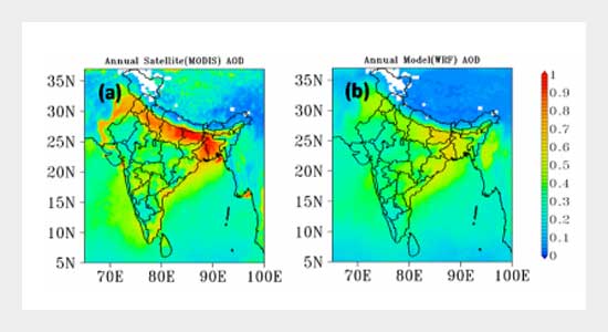
satellite aerosol optical depth AOD PM2.5 mapping
Figure 2: Spatial distribution modeling of satellite-retrieved aerosol column behaviors layered over a dense urban center

C. Meteorological Matrices

  • Parameters: Air Temperature, Relative Humidity, Wind Vector Velocity ($u, v$), Precipitation accumulations, Planetary Boundary Layer Height ($\text{PBLH}$), and Surface Pressure grids.
  • Repositories: ERA5 ECMWF Reanalysis models, NASA MERRA-2 products, or validated regional climate observation stations.

D. GIS Land Use Covariates

  • Features: Line-buffer Road Networks, Distance-to-Axis indices, MODIS/Landsat $\text{NDVI}$, Gridded Population Densities, Corine/Copernicus Land Cover classifications, and SRTM Elevation/Slope terrains.
  • Data Feeds: OpenStreetMap data pools, USGS Landsat archives, ESA Sentinel-2, and WorldPop databases.

9. Operational Methodology Flow

  1. Ingest and cross-verify ground monitoring $\text{PM}_{2.5}$ hourly data sets.
  2. Project, geocode, and anchor target stationary sensor locations into standard spatial coordinate arrays.
  3. Download, clear cloud flags, and composite target satellite imagery bands.
  4. Extract, align, and temporally match raw global meteorological grids.
  5. Construct static regional GIS predictor layers (buffer widths, distance rasters).
  6. Execute point-overlay extractions to isolate all environmental predictor variations at sensor node coordinates.
  7. Train localized machine learning regression engines on the integrated matrices.
  8. Validate model performance via robust spatial hold-out techniques.
  9. Deploy selected top models across continuous regional feature grids.
  10. Render high-resolution spatial heatmaps, raster layers, and hotspot vectors.

10. Spatial Predictor Inventory

Predictor Type Environmental Metric Name Inferred Systemic Control / Influence
Satellite Remote Sensing Aerosol Optical Depth ($\text{AOD}$) Total atmospheric column particulate loading proxy
Biophysical Indices $\text{NDVI}$ (Normalized Difference Vegetation Index) Surface vegetative cover; indicative of natural particulate deposition sinks
Topography Elevation & Slope Profile Terrain barriers; restricts or paths physical pollutant ventilation
Meteorology Dynamics Ambient Temperature Profile Governs local atmospheric stability and chemical reactions
Atmospheric Water Relative Humidity Matrix Triggers hygroscopic particle growth and aggregation processes
Kinematics Wind Speed and Vector Vectoring Controls horizontal transport, dilution, and downwind dispersion
Anthropogenic Proxy Line-Buffer Road Network Density Direct surrogate for primary mobile source fossil fuel emissions
Demographics Gridded Population Density Proxy for domestic energy consumption, localized transport, and exposure footprint
Zoning Profiles Industrial Land Cover Class Points to intense localized point-source manufacturing emissions
Urban Geometry Built-up Impervious Surfaces Reflects surface roughness and microclimatic heat trapping

11. Comparative Algorithmic Implementations

  • Land Use Regression ($\text{LUR}$): Highly transparent, classic parametric approach mapping linear relations; lacks flexibility with sharp atmospheric fluctuations.
  • Random Forest Regressor: Assembles decorrelated decision tree boundaries; manages deep nonlinear dynamics smoothly with high resilience to training noise.
  • Gradient Boosted Trees ($\text{XGBoost}$): Builds sequential loss-minimizing architectures; delivers outstanding predictive accuracy across complex feature maps.
  • Generalized Additive Models ($\text{GAM}$): Bends smooth spline metrics around distinct components, preserving high interpretability without sacrificing adaptive curvature.
  • Deep Neural Networks ($\text{DNN}$): Stacks multi-layered processing units; ideal for digesting exceptionally massive continental datasets with spatial tracking.

12. Statistical Performance Metrics

Model accuracy validation relies heavily on evaluating error variances using standard performance formulas:

$$ \text{RMSE} = \sqrt{ \frac{\sum_{i=1}^{n} (y_i - \hat{y}_i)^2}{n} } $$

$$ \text{MAE} = \frac{\sum_{i=1}^{n} |y_i - \hat{y}_i|}{n} $$

Cross-Validation Frameworks: To prevent performance inflation due to spatial auto-correlation, models are tested using $10$-Fold Cross Validation, Leave-One-Out Cross Validation ($\text{LOOCV}$), and Spatial Block Cross Validation.

13. Technical Operational Workflow

[PM2.5 Sensor Stations] ──► [Quality Assurance & Filtering] ──┐ │ ▼ [Satellite + Climate + GIS Layers] ──► [Spatial Point-Overlay Extraction] │ ▼ [Machine Learning Engine] │ ▼ [Spatial Block Validation] │ ▼ [Continuous Grid Mapping] │ ▼ [High-Res Hotspot Surfaces]

14. Code Execution & Software Requirements

  • GIS Suites: QGIS Desktop, ArcGIS Pro API
  • Language Environments: Python (v3.10+ optimized), R-Statistical Package
  • Core Python Libraries: pandas, geopandas, rasterio, scikit-learn, xgboost, numpy, matplotlib, folium, shapely
  • Cloud Execution: Google Earth Engine Python API, GDAL binary systems

15. Project Target Deliverables

  • Cleaned, query-ready ground monitoring relational spatial database.
  • Standardized environmental landscape GIS predictor rasters.
  • Serialized, deployment-ready machine learning regression model weights.
  • High-resolution $\text{PM}_{2.5}$ continuous regional prediction surfaces.
  • Vectorized localized exposure hotspot directories.
  • Dynamic open-source interactive map engines (Leaflet/Folium frameworks).
  • Relative predictor variable feature importance calculations.
  • Model cross-comparison diagnostics and residual reporting dashboards.
  • Spatial prediction uncertainty maps outlining model variance.
GIS spatial predictor layers environmental monitoring air quality
Figure 3: Multi-pollutant high-resolution spatial prediction grids comparing target particulate matter against gaseous co-pollutants

16. Environmental Policy Applications

The downscaled $\text{PM}_{2.5}$ maps directly support high-tier environmental management, public health risk tracking, smart-city infrastructure zoning, environmental impact assessments ($\text{EIA}$), traffic mitigation policies, green infrastructure routing, and early-warning public health frameworks.

17. Anticipated Outcomes

Fusing spatial ground observation arrays with multi-spectral satellite $\text{AOD}$, atmospheric climate records, and landscape variables is expected to generate continuous, high-fidelity pollution maps. Machine learning architectures like Random Forest and Gradient Boosting ($\text{XGBoost}$) are expected to show superior predictive capability, while Generalized Additive Models ($\text{GAM}$) will provide clear insights into feature behaviors.

18. Scalable Future Enhancements

  • Deployment of near-real-time spatiotemporal prediction pipelines connected directly to numeric weather forecasts.
  • Expansion of multi-task learning models to concurrently map $\text{PM}_{10}$, $\text{NO}_2$, $\text{O}_3$, $\text{SO}_2$, and $\text{CO}$.
  • Integration of advanced Deep Learning networks (Convolutional Neural Networks and Graph Neural Networks) for spatiotemporal predictive mapping.
  • Launch of an automated cloud dashboard providing real-time public exposure alerts and interactive spatial queries.
Meet the Authors
Zacharia Nyambu’s blog features multiple contributors with clear activity status.
Active ✔
πŸ§‘‍πŸ’»
Zacharia Nyambu
Lead Author
Inactive ✖
πŸ‘©‍πŸ’»
Linda Bahati
Co‑Author
Inactive ✖
πŸ‘¨‍πŸ’»
Jefferson Mwangolo
Co‑Author
Inactive ✖
πŸ‘©‍πŸŽ“
Florence Wavinya
Guest Author
Inactive ✖
πŸ‘©‍πŸŽ“
Esther Njeri
Guest Author
Inactive ✖
πŸ‘©‍πŸŽ“
Clemence Mwangolo
Guest Author

Followers