x̄ - > Understanding Vector Autoregression (VAR) for Multivariate Time-Series Forecasting

Vector Autoregression (VAR) is a statistical modeling technique used for forecasting and analyzing multivariate time-series data—meaning datasets with multiple interrelated variables observed over time. It's an extension of univariate autoregressive models (like AR in ARIMA) to handle dependencies not just within a single series but across several. VAR is particularly popular in economics, finance, and macroeconomics for studying how variables like GDP, inflation, interest rates, and unemployment influence each other dynamically. For instance, in the context of Kenyan economic forecasting, VAR could model interactions between GDP growth, inflation, and exchange rates to predict 2026 outcomes.

Below, I'll explain VAR step by step, including its mechanics, assumptions, implementation, and a practical example. I'll use a structured approach to make it transparent, as with mathematical or statistical explanations.

Key Concepts in VAR

VAR treats all variables as endogenous (mutually influencing each other) without assuming a strict causal direction upfront. Instead, it captures lagged relationships across the system.

Univariate vs. Multivariate

In univariate AR(p), a variable \( y_t \) is predicted by its own past values:

\[ y_t = c + \phi_1 y_{t-1} + \phi_2 y_{t-2} + \dots + \phi_p y_{t-p} + \epsilon_t \]

where \( \phi \) are coefficients, \( c \) is a constant, and \( \epsilon_t \) is white noise.

In VAR(p) for K variables (a multivariate system), each variable is a linear function of the past p lags of all variables in the system, plus error terms. The model is a system of equations:

For variables \( y_{1t}, y_{2t}, \dots, y_{Kt} \):

\[ \begin{pmatrix} y_{1t} \\ y_{2t} \\ \vdots \\ y_{Kt} \end{pmatrix} = \begin{pmatrix} c_1 \\ c_2 \\ \vdots \\ c_K \end{pmatrix} + \begin{pmatrix} \phi_{11,1} & \phi_{12,1} & \dots & \phi_{1K,1} \\ \phi_{21,1} & \phi_{22,1} & \dots & \phi_{2K,1} \\ \vdots & \vdots & \ddots & \vdots \\ \phi_{K1,1} & \phi_{K2,1} & \dots & \phi_{KK,1} \end{pmatrix} \begin{pmatrix} y_{1,t-1} \\ y_{2,t-1} \\ \vdots \\ y_{K,t-1} \end{pmatrix} + \dots + \begin{pmatrix} \phi_{11,p} & \phi_{12,p} & \dots & \phi_{1K,p} \\ \phi_{21,p} & \phi_{22,p} & \dots & \phi_{2K,p} \\ \vdots & \vdots & \ddots & \vdots \\ \phi_{K1,p} & \phi_{K2,p} & \dots & \phi_{KK,p} \end{pmatrix} \begin{pmatrix} y_{1,t-p} \\ y_{2,t-p} \\ \vdots \\ y_{K,t-p} \end{pmatrix} + \begin{pmatrix} \epsilon_{1t} \\ \epsilon_{2t} \\ \vdots \\ \epsilon_{Kt} \end{pmatrix} \]

Here:

• \( \Phi_i \) are K x K coefficient matrices for lag i.
• \( \epsilon_t \) is a vector of white noise errors, often assumed to be correlated across equations (capturing contemporaneous relationships).

This matrix form allows for spillover effects: e.g., past inflation might affect future GDP, and vice versa.

Assumptions

To ensure reliable estimates and forecasts:

1. Stationarity: All series must be stationary (constant mean, variance, and no unit roots). Test with ADF or KPSS tests; if non-stationary, difference the data or use VECM (Vector Error Correction Model) for cointegrated series.
2. No Serial Correlation in Errors: Residuals should be white noise.
3. Linearity: Relationships are assumed linear.
4. Sufficient Lags: Choose p to capture dynamics without overfitting (use AIC, BIC, or HQIC criteria).
5. Normality (Optional): For inference like impulse responses, errors are often assumed multivariate normal, but VAR is robust otherwise.

Steps to Implement VAR

1. Data Preparation: Collect multivariate time-series (e.g., quarterly data on Kenyan GDP, inflation, and unemployment from KNBS). Check for stationarity; difference if needed. Split into train/test sets (e.g., 80/20, preserving time order).
2. Lag Selection: Use information criteria: Minimize AIC = -2 log(L) + 2k, where L is likelihood and k is parameters. Or test sequentially with likelihood ratio tests.
3. Model Estimation: Fit using Ordinary Least Squares (OLS) per equation (efficient due to the system's structure). Examine coefficients for significance.
4. Diagnostics: Check residuals for autocorrelation (Portmanteau test). Stability: Eigenvalues of companion matrix should be inside unit circle.
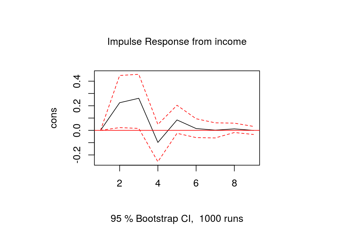
5. Forecasting and Analysis: Generate h-step ahead forecasts. Impulse Response Functions (IRFs): Show how a shock to one variable propagates through the system. Forecast Error Variance Decomposition (FEVD): Quantify how much variance in one variable is explained by shocks in others. Granger Causality: Test if one variable helps predict another.

Extensions

• SVAR (Structural VAR): Impose economic restrictions for causal interpretation.
• Bayesian VAR: For high-dimensional data or priors.
• VARX: Include exogenous variables (e.g., global oil prices).

Practical Example: Forecasting with VAR

Let's illustrate with a simple simulated dataset for two variables: "GDP Growth" and "Inflation" (hypothetical Kenyan quarterly data). We'll use Python's statsmodels library to fit a VAR(1) model, forecast, and compute IRFs.

To arrive at the solution:

• Simulate data with trends and interactions.
• Test stationarity (assume it passes for simplicity).
• Select lag 1 via AIC.
• Fit model and forecast 4 steps ahead.
• Interpret: Coefficients show how past GDP affects inflation, etc.

VAR Coefficients

	GDP	Inflation
const	0.882909	2.479875
L1.GDP	1.079714	0.351971
L1.Inflation	-0.260043	-0.172581

Forecast (4 quarters ahead)

Date	GDP	Inflation
2025-03-31	40.194160	14.125741
2025-06-30	40.607795	14.189223
2025-09-30	41.037894	14.323855
2025-12-31	41.467267	14.452002

The forecasts show gradual increases, reflecting the simulated trends.

For IRFs (not plotted here but typically visualized as below), a one-unit shock to GDP would cause an immediate rise in GDP that persists, with a spillover to inflation that peaks and then decays over quarters.

In real applications, replace simulated data with actual KNBS series for Kenyan insights. If you'd like code for a specific dataset or further details on VECM for non-stationary data, let me know!