Generalized Linear Models Theory
Generalized Linear Models Theory
This is a brief introduction to the theory of generalized linear models. See the "References" section for sources of more detailed information.
Response Probability Distributions
In generalized linear models, the response is assumed to possess a probability distribution
of the exponential form. That is, the probability density of the response Y for continuous response variables, or the probability function for discrete responses, can be expressed as
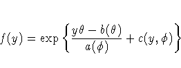
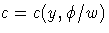
for some functions a, b, and c that determine the specific distribution. For fixed, this is a one-parameter exponential family of distributions. The functions a and c are such that

and
, where w is a known weight for each observation. A variable representing w in the input data set may be specified in the WEIGHT statement. If no WEIGHT statement is specified, wi=1 for all observations.
Standard theory for this type of distribution gives expressions for the mean and variance of Y.
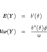
where the primes denote derivatives with respect to

.If

represents the mean of Y, then the variance expressed as a function of the mean is
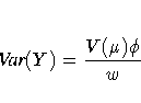
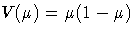
where V is the variance function.
Probability distributions of the response Y in generalized linear models are usually parameterized in terms of the mean
and dispersion parameter

instead of the natural parameter
.The probability distributions that are available in the GENMOD procedure are shown in the following list. The PROC GENMOD scale parameter and the variance of Y are also shown.
The negative binomial distribution contains a parameter k, called the negative binomial dispersion parameter. This is not the same as the generalized linear model dispersion
, but it is an additional distribution parameter that must be estimated or set to a fixed value.
For the binomial distribution, the response is the binomial proportion Y = events/ trials. The variance function is
, and the binomial trials parameter n is regarded as a weight w.
If a weight variable is present,
is replaced with, where w is the weight variable.
PROC GENMOD works with a scale parameter that is related to the exponential family dispersion parameter
instead of with
itself. The scale parameters are related to the dispersion parameter as shown previously with the probability distribution definitions. Thus, the scale parameter output in the "Analysis of Parameter Estimates" table is related to the exponential family dispersion parameter. If you specify a constant scale parameter with the SCALE= option in the MODEL statement, it is also related to the exponential family dispersion parameter in the same way.
Link Function
The mean

of the response in the ith observation is related to a linear predictor through a monotonic differentiable link function g.

Here, xi is a fixed known vector of explanatory variables, and

is a vector of unknown parameters.
Log-Likelihood Functions
Log-likelihood functions for the distributions that are available in the procedure are parameterized in terms of the means
and the dispersion parameter
.The term yi represents the response for the ith observation, and wi represents the known dispersion weight. The log-likelihood functions are of the form
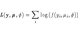
where the sum is over the observations. The forms of the individual contributions
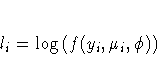
are shown in the following list; the parameterizations are expressed in terms of the mean and dispersion parameters.
For the binomial, multinomial, and Poisson distribution, terms involving binomial coefficients or factorials of the observed counts are dropped from the computation of the log-likelihood function since they do not affect parameter estimates or their estimated covariances.
Maximum Likelihood Fitting
The GENMOD procedure uses a ridge-stabilized Newton-Raphson algorithm
to maximize the log-likelihood function

with respect to the regression parameters.
By default, the procedure also produces maximum likelihood estimates of the scale parameter as defined in the
"Response Probability Distributions"
section for the normal, inverse Gaussian, negative binomial, and gamma distributions.
On the rth iteration, the algorithm updates the parameter vector

with
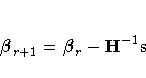
where H is the Hessian
(second derivative) matrix, and s is the gradient
(first derivative) vector of the log-likelihood function, both evaluated at the current value of the parameter vector. That is,
![s = [s_j] = [ \frac{\partial L}{\partial \beta_j} ]](https://www.sfu.ca/sasdoc/sashtml/stat/chap29/images/gmoeq81.gif)
and
![H = [{h_{ij}}] = [ \frac{\partial^2 L} {\partial\beta_i\partial\beta_j} ]](https://www.sfu.ca/sasdoc/sashtml/stat/chap29/images/gmoeq82.gif)
In some cases, the scale parameter is estimated by maximum likelihood. In these cases, elements corresponding to the scale parameter are computed and included in s and H.
If

is the linear predictor for observation i and g is the link function, then

, so that
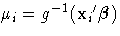
is an estimate of the mean of the ith observation, obtained from an estimate of the parameter vector
.
The gradient vector and Hessian matrix for the regression parameters are given by
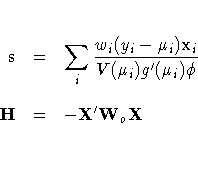
where X is the design matrix, xi is the transpose of the ith row of X, and V is the variance function. The matrix Wo is diagonal with its ith diagonal element
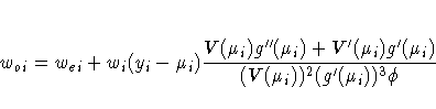
where
The primes denote derivatives of g and V with respect to
.The negative of H is called the observed information matrix.
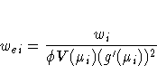
The expected value of Wo is a diagonal matrix We with diagonal values wei. If you replace Wo with We, then the negative of H is called the expected information matrix.
We is the weight matrix for the Fisher's scoring
method of fitting. Either Wo or We can be used in the update equation. The GENMOD procedure uses Fisher's scoring for iterations up to the number specified by the SCORING option in the MODEL statement, and it uses the observed information matrix on additional iterations.
Covariance and Correlation Matrix
The estimated covariance matrix
of the parameter estimator is given by

where H is the Hessian matrix evaluated using the parameter estimates on the last iteration. Note that the dispersion parameter, whether estimated or specified, is incorporated into H. Rows and columns corresponding to aliased parameters are not included in

.
The correlation matrix is the normalized covariance matrix. That is, if

is an element of
, then the corresponding element of the correlation matrix is

,where

.
Goodness of Fit
Two statistics that are helpful in assessing the goodness of fit
of a given generalized linear model are the scaled deviance
and Pearson's chi-square statistic.
For a fixed value of the dispersion parameter
, the scaled deviance is defined to be twice the difference between the maximum achievable log likelihood and the log likelihood at the maximum likelihood estimates of the regression parameters.
Note that these statistics are not valid for GEE models.
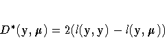
If

is the log-likelihood function expressed as a function of the predicted mean values

and the vector y of response values, then the scaled deviance is defined by
For specific distributions, this can be expressed as
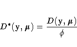
where D is the deviance. The following table displays the deviance for each of the probability distributions available in PROC GENMOD.
In the binomial case, yi=ri/mi, where ri is a binomial count and mi is the binomial number of trials parameter.
In the multinomial case, yij refers to the observed number of occurrences of the jth category for the ith subpopulation defined by the AGGREGATE= variable, mi is the total number in the ith subpopulation, and pij is the category probability.
Pearson's chi-square statistic is defined as
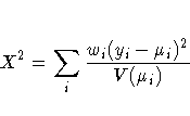
and the scaled Pearson's chi-square is

.
The scaled version of both of these statistics, under certain regularity conditions, has a limiting chi-square distribution, with degrees of freedom equal to the number of observations minus the number of parameters estimated. The scaled version can be used as an approximate guide to the goodness of fit of a given model. Use caution before applying these statistics to ensure that all the conditions for the asymptotic distributions hold. McCullagh and Nelder (1989) advise that differences in deviances for nested models can be better approximated by chi-square distributions than the deviances themselves.
In cases where the dispersion parameter is not known, an estimate can be used to obtain an approximation to the scaled deviance and Pearson's chi-square statistic. One strategy is to fit a model that contains a sufficient number of parameters so that all systematic variation is removed, estimate
from this model, and then use this estimate in computing the scaled deviance of sub-models. The deviance or Pearson's chi-square divided by its degrees of freedom is sometimes used as an estimate of the dispersion parameter
.For example, since the limiting chi-square distribution of the scaled deviance

has n-p degrees of freedom, where n is the number of observations and p the number of parameters, equating D* to its mean and solving for
yields
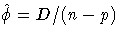
.Similarly, an estimate of
based on Pearson's chi-square X2 is
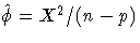
.Alternatively, a maximum likelihood estimate of
can be computed by the procedure, if desired. See the discussion in the "Type 1 Analysis" section for more on the estimation of the dispersion parameter.
Dispersion Parameter
There are several options available in PROC GENMOD for handling the exponential distribution dispersion parameter.
The NOSCALE and SCALE options in the MODEL statement affect the way in which the dispersion parameter is treated. If you specify the SCALE=DEVIANCE option, the dispersion parameter is estimated by the deviance divided by its degrees of freedom. If you specify the SCALE=PEARSON option, the dispersion parameter is estimated by Pearson's chi-square statistic divided by its degrees of freedom.
Otherwise, values of the SCALE and NOSCALE options and the resultant actions are displayed in the following table.
NOSCALE SCALE=value Action present scale fixed at value present not present scale fixed at 1 not present not present scale estimated by ML not present present scale estimated by ML, starting point at value
The meaning of the scale parameter displayed in the "Analysis Of Parameter Estimates" table is different for the Gamma distribution than for the other distributions. The relation of the scale parameter as used by PROC GENMOD to the exponential family dispersion parameter
is displayed in the following table. For the binomial and Poisson distributions,
is the overdispersion parameter, as defined in the "Overdispersion" section, which follows.
In the case of the negative binomial distribution, PROC GENMOD reports the "dispersion" parameter estimated by maximum likelihood. This is the negative binomial parameter k defined in the "Response Probability Distributions" section.
Overdispersion
Overdispersion
is a phenomenon that sometimes occurs in data that are modeled with the binomial or Poisson distributions. If the estimate of dispersion after fitting, as measured by the deviance or Pearson's chi-square, divided by the degrees of freedom, is not near 1, then the data may be overdispersed if the dispersion estimate is greater than 1 or underdispersed if the dispersion estimate is less than 1. A simple way to model this situation is to allow the variance functions of these distributions to have a multiplicative overdispersion factor
.
The models are fit in the usual way, and the parameter estimates are not affected by the value of
.The covariance matrix, however, is multiplied by
, and the scaled deviance and log likelihoods used in likelihood ratio tests are divided by
.The profile likelihood function used in computing confidence intervals is also divided by
.If you specify an WEIGHT statement,
is divided by the value of the WEIGHT variable for each observation. This has the effect of multiplying the contributions of the log-likelihood function, the gradient, and the Hessian by the value of the WEIGHT variable for each observation.
The SCALE= option in the MODEL statement enables you to specify a value of

for the binomial and Poisson distributions. If you specify the SCALE=DEVIANCE option in the MODEL statement, the procedure uses the deviance divided by degrees of freedom as an estimate of
,and all statistics are adjusted appropriately. You can use Pearson's chi-square instead of the deviance by specifying the SCALE=PEARSON option.
The function obtained by dividing a log-likelihood function for the binomial or Poisson distribution by a dispersion parameter is not a legitimate log-likelihood function. It is an example of a quasi-likelihood function. Most of the asymptotic theory for log likelihoods also applies to quasi-likelihoods, which justifies computing standard errors and likelihood ratio statistics using quasi-likelihoods instead of proper log likelihoods. Refer to McCullagh and Nelder (1989, Chapter 9) and McCullagh (1983) for details on quasi-likelihood functions.